Wednesday, December 25, 2013

The best way to use stacked area charts to visualize crazy central bank balance sheets

Before 2008, visualizations of central bank activity largely focused on interest rates. These visualizations were easy to make, just a line graph showing a central bank's target rate and the actual overnight rate, perhaps within a narrow channel bounded at the top by the central bank's lending rate and at the bottom by its deposit rate. The one below, pinched from the Economist, is a decent example.


But then the credit crisis hit. Rates plunged to zero where they have stayed ever since. Central bank policy moved away from conventional manipulation of the short term rate towards more unconventional policies, thus rendering the classic line graph less relevant.

Two of the more important of these new unconventional tools are quantitative and qualitative easing. A good chart must be capable of illustrating the expansion of a central bank's balance sheets (quantitative easing) and contortions within that balance sheet (qualitative easing). In this context, stacked area charts have become the go-to visualization. Not only can they convey the overall size of the central bank's balance sheet and its change over time, but they are also capable of showing the varying contributions of individual stacked areas, giving a sense of movement within the balance sheet.

Because the stacked area chart's large flat areas are typically filled with colours, it reigns as one of the charting universe's more visually stunning specimens, appearing almost Van Gogh-like in its intensity. However, there are a few interesting technical problems with using stacked area charts, two of which I'll describe in this post:

1. Small sums get squished

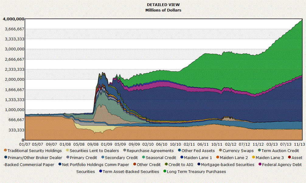
QE has in many cases caused a quadrupling in size of central bank balance sheets. However, pre-QE and post QE periods must share the same scale on a stacked area chart. As a result, pre-QE data tends to get squished into a tiny area at the bottom left of our stacked area chart while post QE data gets assigned to the entire length of the scale. This limits the viewer's ability to make out the various pre-QE components and draw comparisons across time. The chart below, pinched from the Cleveland Fed, illustrates this, the data in 2007 being too squished to properly make out.


The classic way to deal with the squishing of small amounts by large amounts is to use a logarithmic scale. Log scales brings out the detail of the small amounts while reducing the visual dominance of large amounts. The chart below, for instance, illustrates what happens when we graph Apple's share price data on the two different scales.


But log scales don't work with stacked area charts. Below, I've stacked three data series on top of each other and used a logarithmic scale.


Upon a quick visual inspection, you might easily assume that the blue area, Series1, represents the greatest amount of data, the purple the second most, and the yellow the third. But all three represent the same data series: 4, 4, 6, 8, 3, 4. If you look closer and map each series to the logarithmic scale, it becomes evident that all three areas indeed represent the same amount of data. Since the series represented by the blue area happens to be the first series, the log scale assigns it the largest amount of space. If by chance the data represented by the yellow series was first in line, then it would be assigned to the bottom part of the scale and would take up the most area. This is an arbitrary way to go about building a chart.

So applying a log scale to a stacked area chart will cause most people to gather the wrong conclusions. They are interested in the size of the areas, but a log scale assigns equal data series different size areas (or unequal data series the same size area). We've created a mess.

2. Loss of clarity as the stack increases.

Central banks will often have dozens of items on both the asset and liability side of their balance sheets. As each series is stacked on top of the other, volatility in a given series will by amplified across all subsequent stacked layers. This will tend to make it harder for the reader to trace out movements over time in series that are nearer to the top of the stack.

Below I've charted five data series:


Although it may not be apparent to the eye, areas A and E represent the exact same underlying data series. While the eye can easily pick out the gradual rise in A, this simply isn't possible with E. The volatility in the intervening layers B, C, and D make it impossible to pick out the fact that E is a gradually increasing data series, and that A = E.

The fix

My solution to these two problems is an interactive chart. This one shows the Federal Reserve's balance sheet since 2006:


This chart was coded in d3, an awesome javascript library created by Mike Bostock.

The first problem, squished sums, is solved by the ability to create a percent area chart. Try clicking the radio button that says "percent contribution". Rather than each series being assigned an absolute amount, they will now be scaled by their proportional contribution to the total balance sheet. This normalizes pre-QE and post QE data, thereby allowing for comparisons over both periods.

The second problem, the loss of clarity as the stack increases, is solved in two ways. By choosing the unstacked radio button, the chart will drop all data series to a resting position on the x-axis. The volatility of one series can no longer reduce the clarity of another series. This causes some busyness, but the viewer can reduce this clutter by clicking on the legend labels, removing data series that they are not interested until they've revealed a picture that tells the best story.

The loss of clarity can also be solved by leaving the chart in stacked mode, but clicking on legend labels so as to remove the more volatile data series.

There you have it. By allowing the user to 1) shift between stacked, unstacked, and percent contribution modes and 2) add and subtract data, our interactive Fed stacked area chart solves a number of problems that plague non-interactive area charts.

Addendum:

Some interesting random observations that we can pull out of our interactive area chart.

1. If you remove everything but coin (assets), you'll see that every February the Fed shows a spike in coin held. Why is that?
2. Try removing everything but items in the process of collection (assets) and deferred availability cash items (liabilities). Note the dramatic fall in these two series since 2006. The reason for this is that prior to 2001, checks were physically cleared. The Fed leased a few hundred planes which were loaded every night with checks destined for Fed sorting points. Prior to these cheques being settled, the outstanding amount in favour of the Fed was represented as items in process of collection, and those in favour of member banks be deferred availability items. The arrival of digital check technology has reduced the time over which checks remain unsettled, and thus reduced these balance sheet items to a fraction of their previous amounts. Timothy Taylor has a good post on this subject.
3. Unstacking the assets data shows that unamortized discounts/premiums represent the third largest contributor to Fed assets, up from almost nothing back in 2006. Basically, the Fed has been consistently buying large amounts of bonds via QE at a price above their face value. This premium gets added to the unamortized premium category.

Wednesday, December 18, 2013

Tales from the litecoin universe

With cyptocurrencies all the rage these days, I figured I should weigh in. I've done a few dozen posts about the monetary theory behind cryptocoins, so rather than write another, in this post I'm going to describe my somewhat zany experience over the last fourteen or so months with litecoin, one of the bitcoin clones.

Curious about bitcoin, I figured I should gain some practical experience with the medium of exchange on which I planned to write over the next few months. So one cold autumn day in 2012 I bit the bullet and transferred some money to VirtEx, Canada's largest online bitcoin exchange, bought a few coins (a small enough amount that I wouldn't wince if their price fell to $0), and then transferred those coins from my Virtex account to my newly downloaded wallet residing on my laptop. Voilà! I was now officially a bitcoiner.

...which wasn't as exciting as I had anticipated. There was little for me to do with my fresh digital pile of coins. I'm not a huge shopper, and the places where I do buy stuff, like grocery stores, don't accept bitcoin. I don't do drugs, so I couldn't use Silk Road, the now-shuttered online drug marketplace. And I don't gamble, the gambling website SatoshiDice being one of the big drivers of bitcoin transactions. So my coins just sat there in my wallet gathering electronic dust.

Later that autumn I read somewhere that bitcoin had a smaller cryptocurrency cousin called litecoin, which traded for a fraction of the price of bitcoin. Curious, and with little other avenue for my bitcoins, I sent a small chunk of my already small stash of bitcoin to BTC-e, a Russian online exchange specializing in bitcoin-to-litecoin trades, and proceeded to buy some litecoins for around 5 cents each (I can't remember their price in bitcoin). I transferred these to my freshly downloaded litecoin wallet, and voilà, I was also now officially a litecoiner.

Much like my experience with bitcoin, I was tad bit disappointed. As a medium of exchange, litecoin was even less liquid than bitcoin. Whereas a few online sites accepted bitcoin, no one seemed to want litecoin, providing me with little opportunity to play around with my new toys. Along with my bitcoins, my tiny hoard of litecoins gathered dust.

A few weeks later, however, I stumbled on an interesting avenue for my litecoins: an online litecoin-denominated stock exchange called LTC-Global. At the time, it listed around 20-25 stocks and bonds. I gleefully opened an account (which took seconds) to which I transferred about 75% of my stash of litecoins, and started to invest. I use the term "invest" very loosely, even sheepishly. Because the dollar-value of the shares I was purchasing amounted to a few bucks, it was hardly a large enough sum to merit a true analysis of the companies in which I was investing in. I glanced through the summaries of the various listed companies, picked some that I found interesting, and bought their shares. My investments included a website that published litecoin charts, a bond issued by a litecoin miner, a few passthroughs*, and some other companies.

Over the next months I'd get periodic notifications that my companies had paid me dividends. I bought a few more shares here and there, and some of them even rose in value. But when the novelty of this was over, I forgot about my investments. Then in March 2013 litecoin prices really started to race, quickly moving from $0.05 to $0.50. This amounted to a 900% rise since my autumn 2012 entrance into the litecoin universe, a far larger percent return than I'd ever made on my "real life" investments. My stash of litecoin had graduated from the "tiny" to the "smallish" category.

I hastened to LTC-Global to check the price of my investments, and much to my horror discovered that many of them had fallen in value by the exact amount of litecoin's rise. My 900% return was not to be. And as litecoin's price crossed the symbolic $1 mark, the price of my stocks continued to fall! After a few frenzied inquiries posted to the litecoin forums, I was informed by some savvy cryptocoin investors why this was occurring. Many of the companies into which I'd invested my litecoins earned fiat returns. My litecoin chart website, for instance, received advertising income in euros. As litecoin prices exploded, the website continued to earn the same amount of euros, but this equated to a much smaller litecoin equivalent. Thus the price of my stocks in terms of litecoin had declined, though they were still worth the same amount of dollars or euros. Better had I kept my funds in litecoin than ever investing them!

This made me wonder: in a world in which cryptocoins are expected to rise by 900% in a few days (why else would someone hold them), is there any point in investing one's litecoins? The expected return on hoarding far exceeds the return from investing litecoin in companies that by-and-large earn fiat returns. Yes, companies that earn litecoin income will not suffer a fall in share price, but at the time I was making my investments the litecoin universe was so small that few companies earned a pure litecoin revenue stream.

By April, litecoin had advanced another 900% to $5, giving me a return of 9,900% in just a few months. My shares, however, continued to deteriorate in value. To compound the problem, one of the companies I'd blindly invested in turned out to be a scam. I suppose in hindsight I might have guessed that a company called "Moo Cow Mining" might be a poor candidate for investing. The owner of Moo Cow had stopped paying dividends and absconded with the investors' assets. In the bricks & mortar world such actions would have very real consequences, but in the nascent litecoin universe there seemed to be little that could be done except make loud threats on the forums. This caused me some consternation because though my initial investment had been tiny, as litecoin prices advanced from $0.05 to $5 what had been a small scam in real terms quickly became a not-so-small one.

Once again I forgot about my litecoins. Without warning, this September LTC-Global announced it would be shutting its doors. One of the hazards of running an online stock exchange is that it probably breaks hundreds of SEC regulations. No doubt the exchange owners had decided to call it quits before they got in trouble. Worried that my funds might be confiscated or blocked, I quickly logged into my account. My shares had fallen in value (see this post) upon the announcement, but I was still able to sell everything I owned. I limped out of LTC-Global having lost 65% or so of the litecoins I'd invested. I vowed never again to spend away my hoard of coins on silly investments.

This November litecoin prices experienced another buying rush as they rose from $5 to just shy of $50, pushing litecoin up by a ridiculous 99,900% since I'd initially bumbled into them. Although I'd lost a large chunk of my litecoins by investing in stocks, the remaining stash now summed up to an amount that was no longer smallish (but not gigantic, either). Even tiny amounts of capital will grow into something substantial at those sorts of rates of return. Let's not kid ourselves though, this wasn't a canny trade, it was just dumb luck.

Getting out of litecoin isn't an easy task. I'll have to send my coins back to BTC-e where I can exchange them into bitcoin, incurring a 0.05% transaction cost on the deal. Then I have to transfer these bitcoins back to Virtex to buy Canadian dollars, which will exact a fat 2% commission on the trade. Then I'll have to wait a few days for my dollars to be transferred to my bank account. It's a lengthy and expensive process. Alternatively I could try and find someone who makes a market in litecoin, go to their house or a café, and consummate the trade there. But that just sounds awkward.

I also now have the headache of figuring out the tax implications of all of this. Which makes me wonder: how can litecoin and bitcoin ever be useful media-of-exchange if, for tax purposes, one must calculate the capital gain or loss incurred on every exchange? Even if I was able to buy groceries with my litecoin, I'm not sure I'd bother. The laborious process of going through my records in order to determine my capital gain/loss would probably have me reaching for my fiat wallet. The advantage of fiat money is that there are no capital gains taxes or capital loss credits, obviating the need for bothersome calculation.

The tax issue, combined with the general difficulty I experienced buying anything with my litecoins, topped off by the complexity of getting back into fiat all conspire to drive home the point that the main reason to hold litecoins for any period of time isn't because they make great exchange media—it's because they're the best speculative vehicles to hit the market since 1999 Internet stocks. I'll admit straight up that the speculative motive is why I'm still holding my litecoins, the educational motive having receded into the background some time ago. After all, if these little rockets can rise from $0.05 to $50, why not to $500, or $5000? All that's needed is a greater fool. I'm fully aware that the odds are that litecoin's value will fall to zero before $500 is ever reached, but my litecoin gains are so unreal to me that I wouldn't lose any tears if that particular worst-case scenario were to occur.

And it's millions of folks like me who explain the incredible volatility of cryptocoins, since we are the marginal buyers and sellers of the stuff. Since first starting to write this post, litecoin has lost over 60% of its value, falling back to below $20. These speculative-driven spikes and crashes don't seem like a very durable state of affairs to me, at least if cryptocurrencies are to take a more serious role in the world of exchange media. To be useful, an inventory of exchange media should be capable of purchasing the same amount of goods on Wednesday that it bought on Monday, but with cryptocoins one has little clue what tomorrow's purchasing power will be, let alone next week's.

Although I'm skeptical of cryptocoin mania, let me end on a positive note. Cryptocoin 2.0, or stable-value cryptocoins, is probably not too far away. It may take a price crash before they emerge, but I do think that stable value crypto coins will prove to be far better exchange media than the current roster of roller coasters.


*a passthrough is a bit like an ETF. Anyone who invests in a passthrough receives a stream of dividends thrown off by an underlying stock, one that is usually listed on another crypto stock exchange.

Sunday, December 8, 2013

Milton Friedman and moneyness

Steve Williamson recently posted a joke of sorts:
What's the difference between a New Keynesian, an Old Monetarist, and a New Monetarist? A New Keynesian thinks no assets matter, an Old Monetarist thinks that some of the assets matter, and a New Monetarist thinks all of the assets matter.
While I wouldn't try it around the dinner table, what Steve seems to be referring to here is the question of money. New Keynesians don't have money in their models, Old Monetarists have some narrow aggregate of assets that qualify as M, and New Monetarists like Steve think everything is money-like.*

This is a interesting way to describe their differences, but is it right? In this post I'll argue that these divisions aren't so cut and dry. Surprisingly enough, Milton Friedman, an old-fashioned monetarist, was an occasional exponent of the idea that all assets are to some degree money-like. I like to call this the moneyness view. Typically when people think of money they take an either/or approach in which a few select goods fall into the money category while everything else falls into the non-money category. If we think in terms of moneyness, then money is a characteristic that all goods and assets possess to some degree or another.

One of my favorite examples of the idea of moneyness can be found in William Barnett's Divisia monetary aggregates. Popular monetary aggregates like M1 and M2 are constructed by a simple summation of the various assets that economists have seen fit to place in the bin labeled 'money'. Barnett's approach, on the other hand, is to quantify each asset's contribution to the Divisia monetary aggregate according to the marginal value that markets and investors place on that asset's moneyness, more specifically the value of the monetary services that it throws off. The more marketable an asset is on the margin, the greater its contribution to the Divisia aggregate.

Barnett isolates the monetary services provided by an asset by first removing the marginal value that investors place on that asset's non-monetary services, where non-monetary services might include pecuniary returns, investment yields and consumption yields. The residual that remains after removing these non-monetary components equates to the market's valuation of that given asset's monetary services. Since classical aggregates like M1 glob all assets together without first stripping away their various non-monetary service flows, they effectively combine monetary phenomena with non-monetary phenomena—a clumsy approach, especially when it is the former that we're interested in.

An interesting incident highlighting the differences between these two approaches occurred on September 26, 1983, when Milton Friedman, observing the terrific rise in M2 that year, published an article in Newsweek warning of impending inflation. Barnett simultaneously published an article in Forbes in which he downplayed the threat, largely because his Divisia monetary aggregates did not show the same rise as M2. The cause of this discrepancy was the recent authorization of money market deposit accounts (MMDAs) and NOW accounts in the US. These new "monies" had been piped directly into Friedman's preferred M2, causing the index to show a discrete jump. Barnett's Divisia had incorporated them only after adjusting for their liquidity. Since neither NOW accounts nor MMDAs were terribly liquid at the time—they did not throw off significant monetary services—their addition to Divisia hardly made a difference. As we know now, events would prove Friedman wrong since the large rise in M2 did not cause a new outbreak of inflation.**

However, Friedman was not above taking a moneyness approach to monetary phenomenon. As Barnett points out in his book Getting it Wrong, Friedman himself requested that Barnett's initial Divisia paper, written in 1980, include a reference to a passage in Friedman & Schwartz's famous Monetary History of the United States. In this passage, Friedman & Schwartz discuss the idea of taking a Divisia-style approach to constructing monetary aggregates:
One alternative that we did not consider nonetheless seems to us a promising line of approach. It involves regarding assets as joint products with different degrees of "moneyness" and defining the quantity of money as the weighted sum of the aggregate value of all assets, the weights varying with the degree of "moneyness".
F&S go on to say that this approach
consists of regarding each asset as a joint product having different degrees of "moneyness," and defining the quantity of money as the weighted sum of the aggregate value of all assets, the weights for individual assets varying from zero to unity with a weight of unity assigned to that asset or assets regarded as having the largest quantity of "moneyness" per dollar of aggregate value.
There you have it. The moneyness view didn't emerge suddenly out of the brains of New Monetarists. William Barnett was thinking about this stuff a long time ago, and even an Old Monetarist like Friedman had the idea running in the back of his mind. And if you go back even further than Friedman, you can find the idea in Keynes & Hayek, Mises, and as far back as Henry Thornton, who wrote in the early 1800s. The moneyness idea has a long history.


* Steve on moneyness: "all assets are to some extent useful in exchange, or as collateral. "Moneyness" is a matter of degree, and it is silly to draw a line between some assets that we call money and others which are not-money."

...and on old monetarists: "Central to Old Monetarism - the Quantity Theory of Money - is the idea that we can define some subset of assets to be "money". Money, according to an Old Monetarist, is the stuff that is used as a medium of exchange, and could include public liabilities (currency and bank reserves) as well as private ones (transactions deposits at financial institutions)."

** See Barnett, Which Road Leads to Stable Money Demand?

Saturday, November 30, 2013

The three lives of Japanese military pesos

1942 Japanese Invasion Philippines Peso with a JAPWANCAP Stamp

In his reply to Mike Sproul, Kurt Schuler brings up the question of the determination of the value of a very peculiar kind of money: military currency. Curious, I investigated one example of such money, Japanese-issued "invasion money" in Philippines both during and after World War II. As best I can tell, the mechanism by which the value of these military notes has been mediated has gone through three different phases, each of them teaching us something interesting about money.

In January 3, 1942, a few weeks after successfully invading Philippines, the Japanese Commander-in-Chief announced that occupying forces would henceforth use military-issued currency as legal tender. Notes were to circulate at par with existing Philippines "Commonwealth" Pesos. Since this military scrip was not directly convertible into existing pesos, the trick to get it to circulate at par can probably be found in the tersely titled proclamation Acts punishable by death which, among seventeen acts that could result in loss of life, listed the thirteenth as:
(13) Any person who counterfeits military notes; refuses to accept them or in any way hinders the free circulation of military notes by slanderous or seditious utterances.
This is a great example of a Warren Mosler fiat money. According to Mosler, the state's requirement that citizens discharge their tax obligation with a certain intrinsically worthless medium on pain of being shot in the head is sufficient to give that medium a positive value. Likewise, requiring citizens to use the same medium in the course of regular payments and accept it to discharge debts, all on pain of death, would probably have promoted a positive value for intrinsically worthless paper.

Over time, those bits of "forced" paper will enjoy constant purchasing power as long as the issuer withdraws excess currency or adds it when desired. This is the quantity theory of money.

By 1943, however, it seems that the Japanese occupying forces, now being pushed back by the Allied forces, were desperately issuing excess notes to pay for operations. The Filipino monetary system proceeded to run smack dab into Gresham's law. The unit of account, the peso, was defined in terms of two different media—original pesos and military pesos. This meant that debtors could choose to discharge their debts with either. However, if one was perceived to be more valuable than the other, this superior medium would be hoarded and the inferior one used to pay off the debt. Legacy pesos had completely disappeared from circulation by 1943—only war pesos were being used to discharge debts and pay for goods, a decent indicator that the value of Japanese invasion pesos had fallen below that of original pesos. Bad money had chased out the good. (See [1] and [2] for evidence of Gresham's law)

Through 1944 and 1945, the war peso would endure extreme inflation. 10P had been the largest denomination in 1942. The military introduced 100P, 500P, and 1000P notes in subsequent years. In Neil Stephenson's Cryptonomicon, a wide-ranging historical/science fiction novel filled with monetary themes, there's an interesting passage in which Japanese soldier Goto Dengo describes the use of military scrip, probably sometime in 1943 or 1944:
The owner comes over and hands Goto Dengo a pack of Lucky Strikes and a book of matches. "How much?" says Goto Dengo, and takes out an envelope of money that he found in his pocket this morning. He takes the bills out and looks at them: each is printed in English with the words THE JAPANESE GOVERNMENT and then some number of pesos. There is a picture of a fat obelisk in the middle, a monument to Jose P. Rizal that stands near the Manila Hotel.
The proprietor grimaces. "You have silver?"
"Silver? Silver metal?"
"Yes," the driver says.
"Is that what people use?" The driver nods.
"This is no good?" Goto Dengo holds up the crisp, perfect bills.
The owner takes the envelope from Goto Dengo’s hand and counts out a few of the largest denomination of bills, pockets them, and leaves.
Goto Dengo breaks the seal on the pack of Lucky Strikes, raps the pack on the tabletop a few times, and opens the lid.
Japanese invasion currency, already being well on its way to being repudiated, would become completely worthless upon Japan's unconditional surrender in 1945.

Well, not entirely valueless. The second chapter in the life of military scrip begins with The Japanese War Notes Claimants Association of the Philippines, or JAPWANCAP. Formed in 1953 on behalf of Filipinos left holding stranded quantities of worthless Japanese invasion money, JAPWANCAP's mission was to hold both the US and Japanese government's liable for the redemption of war currency (the US had also issued counterfeit Japanese military currency). So while pesos had been valued prior to the war's end upon pain of death, and their value regulated by limiting the quantity outstanding, those same pesos were now valued on the margin as a liability of their issuer. Given the possibility of redemption, an old invasion note was worth more than zero.

Was JAPWANCAP successful? While the case was heard in a United States Court of Claims in 1967, it was thrown out on a technicality, the statute of limitations having had passed. Put simply, the court would not hear a claim that had not been filed within six years of that claim first being accrued, and in JAPWANCAP's case many more years than that had already passed.

This makes one wonder, if Filipinos in 1953 were already convinced that Japanese invasion pesos were the liability of the issuer, and therefore redeemable in some quantity of yen or dollars, did that same motivation also lead them to originally accept new military pesos in 1942? To what degree was the initial acceptance of pesos driven by the threat of force (& subsequent changes in value regulated by their quantity), and to what degree was their value dictated by their status as a liability of a well-backed issuer? That's a question we can never be entirely sure of. But while the force/quantity theory story fits the facts, the liability story does too. The military peso's inflation, for instance, can be attributed to the rising quantity of money, but also to the increasing likelihood of Japan losing the war, a loser's liability's being worth far less than a winner's.

Which brings us to the third chapter in the evolution of Japanese military pesos. Nowadays you can buy the notes on eBay for a few bucks. Their value is no longer dictated by gunpoint, nor by their liability nature, but their existence as a unique commodity, much like gold, bitcoin, or some rare antique.


To learn more, here is a paper called "Financing Japan’s World War II occupation of Southeast Asia"

Note: I will be posting sparsely over the next two months, probably once every two weeks.

Wednesday, November 20, 2013

Friends, not enemies: How the backing and quantity theories co-determine the price level


Kurt Schuler was kind enough to host a Mike Sproul blog post, which I suggest everyone read.

I think Mike's backing theory makes a lot of sense. Financial analysis is about kicking the tires of a issuer's assets in order to arrive at a suitable price for the issuer. If we can price stocks and bonds by analyzing the underlying cash flows thrown off by the issuer's assets, then surely we can do the same with bank notes and bills. After all, notes and bills, like stocks and bonds, are basically claims on a share of firm profits. They are all liabilities. Understand the assets and you've understood the liability (subject to the fine print, of course), how much that liability should be worth in the market, and how its price should change.

Mike presents his backing theory in opposition to the quantity theory of money. But I don't think the two are mutually exclusive. Rather, they work together to explain how prices are determined. By quantity theory, I mean that all things staying the same, an increase in the quantity of a money-like asset leads to a fall in its price.

We can think of a security's market price as being made up of two components. The first is the bit that Mike emphasizes: the value that the marginal investor places on the security's backing. "Backing" here refers to the future cash flows on which the security is a claim. The second component is what I sometimes refer to as moneyness—the additional value that the marginal investor may place on the security's liquidity, where liquidity can be conceived as a good or service that provides ongoing benefits to its holder. This additional value amounts to a liquidity premium.

Changes in backing—the expected flow of future cash flows—result in a rise or fall in a security's overall price. Mike's point is that if changes in backing drive changes in stock and bond prices, then surely they also drive changes in the price of other claims like bank notes and central bank reserves. Which makes a lot of sense.

But I don't think that's the entire story. We still need to deal with the second component, the security's moneyness. Investors may from time to time adjust the marginal value that they attribute to the expected flow of monetary services provided by a security. So even though a money-like security's backing may stay constant, its price can still wobble around thanks to changes in the liquidity premium. Something other than the backing theory is operating behind the scenes to help create prices.

The quantity theory could be our culprit. If a firm issues a few more securities for cash, its backing will stay constant. However, the increased quantity now in circulation will satisfy the marginal buyer's demand for liquidity services. By issuing a few more securities, the firm meets the next marginal buyer's demand, and so on and so on. Each issuance removes marginal buyers of liquidity from the market, reducing the market-clearing liquidity premium that the next investor must pay to enjoy that particular security's liquidity. In a highly competitive world, firms will adjust the quantity of securities they've issued until the marginal value placed on that security's liquidity has been reduced/increased to the cost of maintaining its liquidity, resulting in a rise or fall in the price of the security.

This explains how the quantity theory works in conjunction with the backing theory to spit out a final price. In essence, the quantity theory of money operates by increasing or decreasing the liquidity premium, Mike's backing theory takes care of the rest.


P.S. Kurt Schuler's response to Mike.

Sunday, November 17, 2013

BlackBerry needs a Draghi moment


The Blackberry debacle reminds me of another crisis that has passed by the wayside—remember the eurozone's Target2 crisis? The same sorts of forces that caused the Target2 crisis, which was really an intra-Eurosystem bankrun, are also at work in the collapse of Blackberry, which can also be thought of an intra-phone run. By analogy, the same sort of actions that stopped the Target2 crisis should be capable of halting the run on Blackberry phones.

Target2 is the ECB mechanism that allows unlimited amounts of euros held in, say, Greek banks to be converted at par into euros at, say, German banks, and vice versa. As the European situation worsened post credit-crisis, people began to worry about a future scenario in which Ireland, Greece, Spain, Italy, and/or Portugal might either leave the euro or be ejected. If exit occurred, it was expected that these new national currencies, drachmas, punts, and lira, would be worth a fraction of what the euro was then trading for.

The chance that this future "bad" scenario might happen accelerated what had been a steady outflow of deposits from the GIIPS into an all-out run—after all, why would anyone risk being stuck with a Greek euro that might be worthless tomorrow when they could costlessly switch them into a German, Dutch, or Finnish euro today at rate of 1:1? The resulting market process was a reflexive one. Mounting Target2 imbalances caused by the run increased the likelihood of a breakup scenario, amplifying the run and creating even greater imbalances.

What ended the run? ECB President Mario Draghi stepped to the plate in a July 26, 2012 speech and directly addressed what he referred to as convertibility risk.
Within our mandate, the ECB is ready to do whatever it takes to preserve the euro. And believe me, it will be enough... [link]
Draghi's comments, as Gavyn Davies then pointed out, amounted to an explicit commitment to backstop the GIIPS to whatever extent was necessary to quell any fears of euro departure. In essence, he took the future "bad" state of the world in which exit occurred and crushed it under his foot. As this chart shows (this one is good too), the massive inflows into German banks and outflows from the periphery were halted almost to the day of Draghi's speech. After all, if the ECB now guaranteed that Greece and the rest were to remain moored to the union, then a GIIPS Euro was once again equally as good as German, Dutch, or Finnish one.

Blackberry is also encountering a run of sorts as Blackberry users flee into competing phones. In normal times, cell phone brands are like euros—they are homogeneous goods that perform the same task. However, just as fears that Greek euros might one day cease to exist inspired a run into German euros, fears that Blackberry's product line might be discontinued (and left unsupported) are causing an all-out run into iPhones and Androids. After all, why risk being stuck with a legacy Blackberry when, come the expiration of your existing contract, you can costlessly switch into a competing phone that has all the same features, the manufacturer of which is sure to exist a few years from now? Take Pfizer for instance, which recently told its employees that "in response to declining sales, the company [Blackberry] is in a volatile state. We recommend that BlackBerry clients use their BlackBerry devices and plan to migrate to a new device at normal contract expiration."

Blackberry desperately needs to have a Draghi moment whereby the future "bad" scenario—firm dissolution and product discontinuance—is crushed and exorcised, thus putting an end to the run. A long-term commitment with a show of muscle is needed. Has this occurred yet? Last month the company came out with an advertisement titled "You can continue to count on us", highlighting the company's formidable stash of cash and clean balance sheet. A start for sure, but no muscle. Last week, however, investor Prem Watsa stepped forward to play the role of Draghi, recapitalizing Blackberry (along with other investors) to the tune of $1 billion. The infusion should give the firm the raw cash to stay in operation for another few quarters. Is Watsa's line-in-the-sand enough to stop phone buyers from fleeing? Or will shoppers continue to spurn BlackBerry on the chance that more billions will be needed, and Watsa unlikely to stump up the cash? The Globe and Mail quotes Watsa, who gives an accurate account of Blackberry's conundrum:
"Why would you buy a BlackBerry system or a BlackBerry phone if you think the company is not going to survive? Well, that’s out. BlackBerry is here to stay,” he said, adding “There’s no question”
There you go, it's a Draghi moment of sort. Substitute "Blackberry" with "Greek Euro" and you have the exact same message that Draghi conveyed to markets last year in his successful halt of the intra-Eurosystem bank run. Like Greek euros, BlackBerries are presumably here to stay.

The difference between Draghi and Watsa is that a central banker can create any amount of money he or she requires—Watsa, who doesn't have his own printing press, is a little more constrained. However, if Watsa has managed to muster up a true Draghi moment, one that is sufficiently credible with smartphone buyers so as to crush the future "bad" scenario out of existence, then the intra-phone run that has plagued Blackberry is probably over and today may be a good time to own shares.


PS: I don't own BlackBerry shares, but am considering it. Dissuade me if you can, commenters.

Tuesday, November 12, 2013

1,682 days and all's well


1,682 is the number of days that the Dow Jones Industrial Average has spent rising since hitting rock bottom back in March 6, 2009.

It also happens to be the number of days between the Dow's July 8, 1932 bottom and its March 10, 1937 top. From that very day the Dow would begin to decline, at first slowly, and then dramatically from August to November when it white-knuckled almost 50%, marking one of the fastest bear market declines in history.

Comparisons of our era to 1937 seems apropos. Both eras exhibit near zero interest rates, excess reserves, and a tepid economic recovery characterized by chronic unemployment. Are the same sorts of conditions that caused the 1937 downturn likely to arise 1,682 days into our current bull market?

The classic monetary explanation for 1937 can be found in Friedman & Schwartz's Monetary History. Beginning in August 1936, the Fed announced three successive reserve requirement increases, pushing requirements on checking accounts from 13% to 26% (see chart below). The economy began to decline, albeit after a lag, as banks tried vainly to restore their excess reserve position by reducing lending and selling securities. A portion of the reserve requirement increase was rolled back on April 14, 1938, too late to prevent massive damage being done to the economy. The NBER cycle low was registered in June of that year.


Friedman & Schwartz's second monetary explanation for 1937 has been fleshed out by Douglas Irwin (pdf)(RePEc). In December 1936, FDR began to sterilize foreign inflows of gold and domestic gold production (see next paragraphs for the gritty details). This effectively froze the supply of base money, which had theretofore been increasing at a rate of 15-20% or so a year. Tight money, goes the story, caused the economy to plummet, a decline mitigated by FDR's announcement on February 14, 1938 to partially desterilize (and therefore allow the base to increase again, with limits), further mitigated by an all-out cancellation of the sterilization campaign that April.

Here are the details of how sterilization worked. (If you find the plumbing of central banking tedious, you may prefer to skip to the paragraph that begins with ">>" — I'll bring the 1937 analogy back to 2013 after I'm done with the plumbing). In the 1920s, the supply of base money could be increased in several ways. First, Fed discounting could do the trick, whereby new reserves were lent out upon appropriate collateral. The Fed could also create new reserves and buy either government securities in the open market or bankers acceptances. Lastly, gold was often sold directly to the Fed in exchange for base money. After 1934, all but the last of these four avenues had been closed. Both the Fed's discount rate and its buying rate on acceptances was simply too high to be attractive to banks, and the practice of purchasing government securities on the open market had long since petered out. Only the gold avenue remained.

New legislation in 1934 meant that all domestic gold and foreign gold inflows had to be sold to the Treasury at $35/oz. The Secretary of the Treasury would write the gold seller a cheque drawn on the Treasury's account at the Fed, reducing the Treasury's balance. The Treasury would then print off a gold certificate representing the number of ounces it had purchased, deposit the certificate at the Fed, and have the Fed renew its account balance with brand-spanking new deposits. Put differently, gold certificates were monetized. As the Treasury proceeded to pay wages and other expenses out of its account during the course of business, these new deposits were injected into the banking system.

You'll notice that by 1934 the Treasury, and not the Fed, had become responsible for increasing the base money supply, a situation that may seem odd to us today. As long as the Treasury Secretary continuously bought gold and took gold certificates representing those ounces to the Fed to be monetized, the supply of base money would increase one-for-one as the Treasury drew down its account at the Fed.

The Treasury's decision to sterilize gold inflows in December 1936 meant that although it would continue to purchase gold, it would cease bringing certificates to the Fed to be monetized. The Treasury would pay for each newly mined gold ounce and incoming foreign ounces by first transferring tax revenues and/or the proceeds of bond issuance to its account at the Fed. Only then could it afford to make the payment. Whereas the depositing of gold certificates by the Treasury had resulted in the creation of new base money, neither the transfer of tax revenues nor the proceeds of bond issuance to the Treasury's account would have resulted in the creation of new base.

FDR's sterilization campaign therefore froze the base. Gold was kept "inactive" in Treasury vaults, as Friedman & Schwartz would describe it. The moment the sterilization campaign was reversed (partially in February 1938, and fully in April), certificates were once again monetized, the base began to expand again, and a rebound in stock prices and the broader economy followed not long after.

>> Let's bring this back to the present. Before 2008 the Fed typically increased the supply of base money as it defended its target for the federal funds rate. The tremendous glut of base money created since 2008 and the introduction of interest-on-reserves has given the Fed little to defend, thus shutting the traditional avenue for base money increases. Just as the gold avenue became the only way to increase the base in 1936, quantitative easing has become the only route to get base money into the banking system. With that analogy in mind, FDR's 1936 sterilization campaign very much resembles an end to QE, doesn't it? Both actions freeze of the monetary base. Likewise, last September's decision to avoid tapering is analogous to the 1938 decision to cease sterilization (or to "desterilize") —both of these decisions unfreeze the base.

Who cares if the base is frozen? After all, in 1937 and today, any pause in base creation won't change the fact that there is already a tremendous glut in reserves. A huge pile of snow remains a huge pile, even after it has stopped snowing.

One reason that desterilization and ongoing QE might be effective is because they shape expectations about future monetary policy, and these expectations are acted upon in the present. For instance, say that the market expects the glut of base money to be removed five years in the future. Only then will reserves regain their rare, or "special" status. While a sudden announcement to taper or sterilize will do little to reduce the present glut, it might encourage the market to move up the expected date of the glut's removal by a year or two. Which will only encourage investors in the present to sell assets for soon-to-be rare reserves, causing a deflationary decline in prices. On the other hand, a renewed commitment to QE or desterilization may extend glut-expectations out another few years. This promise of an extended glut period pushes the prospect that reserves might once again be special even further down the road. With the return on base money having been reduced, current holders of the base will react by trying to offload their stash now—thus causing a rise in prices in the present.

If the monetary theories about the 1937 recession are correct, it is no wonder then that 1,682 days into our current bull market investors seem to be so edgy about issues like tapering. Small changes in current purchasing policies may have larger effects on markets than we would otherwise assume thanks to the intentions they convey about future policy.

QE is effective insofar as it is capable of pushing market expectations concerning the future removal of the base money glut ever farther into the future. But once that lift-off point has been pushed so far off into the distant future (say ten years) that the discounted value of going further is trivial, more QE will have minimal impact.

If QE is nearing the end of its usefulness, what happens if we are hit by a negative shock in 2014? Typically when an exogenous shock hits the economy and lowers the expected return on capital, the Fed will quickly reduce the return on base money in order to ensure that it doesn't dominate the return on capital. If the base's return is allowed to dominate, investors will collectively race out of capital into base money, causing a crash in capital markets. The problem we face today is that returns on capital are currently very low and nominal interest rates near zero. Should some event in 2014 cause the expected return on capital to fall below zero, there is little room for the Fed to reduce the return on base money so as to prevent it from dominating the return on capital—especially with interest-on-reserves unable to fall below zero and QE approaching irrelevance. Come the next negative shock, we may be doomed to face an unusually sharp and quick crash in asset prices (like 1937) as the economy desperately tries to adapt to the superior return on base money.

So while I am still somewhat bullish on stocks 1,682 days into the current bull market, I am worried about the potential for contractionary spirals given that we are still at the zero-lower bound. I'm less worried about the Fed implementing something like a 1937-style sterilization campaign. Incoming Fed chair Janet Yellen is well aware of the 1937 event and is unlikely to follow the 1937 playbook. Writes Yellen:
If anything, I’m more concerned that we will be tempted to tighten policy too soon, thereby aborting recovery. That’s just what happened in 1936 when, following two years of robust recovery, the Fed tightened policy because it was worried about large quantities of excess reserves in the banking system. The result? In 1937, the economy plunged back into a deep recession.  -June 30, 2009 [link


Other recent-ish commentary on the 1937 analogy include Paul Krugman, Francois Velde (pdf), Scott Sumner, Lars Christensen, Christina Romer, Charles Calomiris (pdf), Business Insider, and David Glasner.

Thursday, November 7, 2013

Rates or quantitites or both


Roaming around the econ blogosphere, I often come across what seems to be a sharp divide between those who think monetary policy is all about the manipulation of interest rates and those who think it comes down to varying the quantity of base money. Either side get touchy when the other accuses its favored monetary policy tool, either rates or quantities, of being irrelevant. From my perch, I'll take the middle road between the two camps and say that both are more-or-less right. Either rates, or quantities, or both at the same time, are sufficient instruments of monetary policy. Actual central banks will typically use some combination of rates and quantities to hit their targets, although this hasn't always been the case.

Just to refresh, central banks carry out monetary policy by manipulating the total return that they offer on deposit balances. This return can be broken down into a pecuniary component and a non-pecuniary component. By varying either the pecuniary return, the non-pecuniary return, or both, a central bank is able to create a disequilibrium, as Steve Waldman calls it, which can only be re-equilibrated by a rise or fall in the price level. If the net return on balances is sweetened, banks will flee assets for balances, causing a deflationary fall in prices. If the return is diminished, banks will flock to assets from balances, pushing prices higher and causing inflation.

The pecuniary return on central bank balances is usually provided in the form of a promise to pay interest, or interest on reserves.

The non-pecuniary return, or convenience yield, is a bit more complicated. I've talked about it before. In short, it's sorta like a consumption return. Because central bank balances are useful in settling large payments, and they are rare, banks find it convenient to hold a small quantity of them as a precaution against uncertain events. This unique convenience provided by scarce balances is consumed over time, much like a fire extinguisher's property as a fire-hedge is consumed though never actually mobilized. By increasing or decreasing the quantity of rare balances, a central banker can decrease or increase the value that banks ascribe to this non-pecuniary return.

Now some examples.

The best example of a central bank resorting solely to the quantity tool in order to execute monetary policy is the pre-2008 Federal Reserve. Before 2008, the Fed was not permitted to pay interest on reserves (IOR). This meant that the only return that Fed balances could offer to banks was a non-pecuniary convenience yield, a point that I described here. By adding to or subtracting from the quantity of balances outstanding the Fed could alter their marginal convenience, either rendering them less convenient so as to drive prices up, or more convenient so as to push prices down.

The Bank of Canada is a good example of a central bank that uses both a quantity tool AND an interest rate tool, though not always both at the same time. Since 1991, according to Mark Sadowski, the BoC has paid interest to anyone who holds overnight balances. This is IOR, although in Canada we refer to it as the deposit rate. In addition to paying this pecuniary return, BoC balances also yield a non-pecuniary return. Banks who hold balances enjoy a stream of consumptive returns, or a convenience yield, that stems from both the rarity of BoC balances and their exceptional liquidity.

The best way to "see" how these two returns might be decomposed is by looking at the short term rental market for Bank of Canada balances, or the overnight market. In Canada, this rate is called CORRA, or the Canadian overnight repo rate. A bank will only part with BoC balances overnight if a prospective borrower promises to sufficiently compensate the lending bank for foregone returns. Assuming that the Bank of Canada's deposit rate is 2%, a potential lender will need to be compensated with a pecuniary return of at least 2% in order to dissuade them from socking away balances at the BoC's deposit facility.

The lender will also need to be compensated for doing without the non-pecuniary return on balances. If the overnight lending rate, CORRA, is 2.25%, then we can back out the rate that a lender expects to earn for renting out the non-pecuniary services provided by balances. Since the lender of balances receives the overnight rate of 2.25% from the borrowing bank, and 2% of this can be considered as compensation for foregoing the 2% pecuniary return on balances, that leaves the remaining 0.25% as compensation to the lender for the loss of the non-pecuniary return.

So in our example, the pecuniary and non-pecuniary returns on BoC balances are 2% and 0.25% respectively, for a total return of 2.25%.

The Bank of Canada meets each six weeks, as Nick Rowe points out, upon which it promises to provide banks with a given return on settlement balances, say 2.25%, for the ensuing six week period. When it next meets, the Bank will  introduce whatever changes to this return that are considered necessary for it to hit its monetary policy targets. The BoC can modify the return by changing either the pecuniary component of the total return, the non-pecuniary component, or some combination of both.

Say it modifies only the non-pecuniary component while leaving their pecuniary return untouched. For instance, with the overnight rate trading at 2.25%, the BoC might announce that it will conduct some open market purchases in order to increase the quantity of balances outstanding, while keeping the deposit rate fixed at 2%. By rendering balances less rare, purchases effectively reduce the non-pecuniary return on balances. As a reflection of this shrinking return, the overnight rate may fall a few basis point, or it may fall all the way to 2%. Whatever the case, the rate at which banks now expect to be compensated for foregoing the non-pecuniary return on balances has been diminished. Banks will collectively try to flee out of overpriced clearing balances into assets, pushing up the economy's price level until balances once again provide a competitive return. This sort of pure quantity effect is the story that the quantities camp likes to emphasize.

The story told by the quantities camp is exactly how the BoC loosened policy between April 2009 and May 2010. At the time, the BoC injected $3 billion in balances *without* a corresponding decrease in the deposit rate. The overnight rate fell from 0.5% until it rubbed up against the 0.25% deposit rate. The lack of a gap between the overnight rate and the deposit rate indicated that the injection had reduced the overnight non-pecuniary return on balances to 0%. After all, if lenders still expected to be compensated for forgoing the non-pecuniary return on balances, they would have required that the overnight rate be above the deposit rate.

The BoC's decision to reduce the overnight non-pecuniary return on balances to 0% would have generated a hot potato effect as banks sold off lower-yielding BoC balances for higher-yielding assets, thus pushing prices higher. A change in quantities, not rates, was responsible for the April 2009 to May 2010 loosening.

Likewise, in June 2010, the BoC tightened by using quantities, not rates. Open market sales sucked the $3 billion in excess balances back in, thereby increasing the marginal convenience yield on central bank balances. The deposit rate remained moored at 0.25%, but the overnight rate jumped back to 0.5%, indicating that the overnight non-pecuniary return on balances had increased from 0% to 0.25%. This sweetening in the return on balances would have inspired a portfolio adjustment away from low-yielding assets into high-yielding central bank balances, a process that would have continued until asset prices had fallen far enough to render investors indifferent once again along the margin between BoC deposits and assets. Once again quantities, not rates, did all the hard work.

While the BoC chose to tighten in June 2010 by changing quantities, it could just as easily have tightened by changing rates. For instance, if it had increased the deposit rate to 0.5% while keeping quantities constant, then the net return on balances would have risen to 0.5%, the same return that was generated in the last paragraph's quantities-only scenario. This sweetening in the return on balances would have caused the exact same chain of portfolio adjustments and falling asset prices that the quantities-only scenario caused.

Alternatively, the BoC could have tightened through some combination of quantities AND rates. It might have increased the deposit rate from 0.25% to 0.4%, and then conducted just enough open market sales to increase the non-pecuniary return on balances from 0% to 0.1%, for a total combined return of 0.5%. The ensuing adjustments would have been no different than if tightening had been accomplished by quantities-only or rates-only.

Putting aside the period between April 2009 and June 2010, does the Bank of Canada normally execute monetary policy via rates or quantities? A bit of both, I'd say. At the end of a six week period, say that the Bank wishes to tighten. It typically tightens by announcing a 0.25% rise in its target for the overnight rate combined with a simultaneous 0.25% rise in the deposit rate. The overnight rate, or the rental rate on clearing balances, will typically rise immediately by 0.25%, reflecting the sweetened return on balances.

Did rates or quantities do the heavy lifting in pushing up the return on balances? Put differently, was it the threat that open market sales might increase the convenience yield on balances that tightened policy, or was it the improvement in the deposit rate? I'd argue that the immediate punch would have been delivered by the change in the deposit rate. CORRA, the rental rate on balances, jumped because overnight borrowers of BoC balances were suddenly required to compensate lenders for the higher pecuniary rate being offered by the BoC on its deposit facility. Quantities don't enter into the picture at all, at least not at first. The rates-only camps seems to be the winner.

However, as the ensuing six-week period plays out, market forces will push the rental rate on BoC balances (CORRA) above or below the Bank's target, indicating an improvement or diminution of the total return on balances. The BoC has typically avoided any incremental variation of the deposit rate to ensure that the rental rate, or return on balances, stays true to target over the six week period. Rather, it has always used quantity changes (or the threat thereof) to modify the non-pecuniary return on balances during that period, thereby steering the rental rate back towards target. First rates, and then quantities, conspire together to create Canadian monetary policy.

To sum up, the Bank of Canada's monetary policy is achieved, it would seem, through a complex combination of rate and quantity adjustments. The rates vs. quantities dichotomy that sometimes pops up on the blogosphere simplifies what is really a more nuanced story. Monetary policy can certainly be carried out by focusing on quantity adjustments to the exclusion of rate adjustments (as was the case with the pre-2008 Fed) or vice versa . However, modern central banks like the Bank of Canada use rates, quantities, and some combination of both, to achieve their targets.


Note: The elephant in the room is the zero-lower bound. But the zero lower bound needn't prevent rates or quantities from exerting an influence on prices. On the rates side of the equation, the adoption of a cash-penalizing mechanism along the lines of what Miles Kimball advocates would allow a central bank to safely push rates below zero. As for the quantity side of the equation,  the threat of Sumnerian permanent increases in the monetary base may not be able to reduce the overnight non-pecuniary return on balances once that rate has hit zero, as Steve Waldman points out... but they can certainly reduce the future non-pecuniary returns provided by balances. Reductions in future non-pecuniary returns should be capable of igniting a hot potato effect, albeit a diminishing one, out of balances and into assets.

Friday, November 1, 2013

An ode to illiquid stocks for the retail investor


Today's go-to advice for the small retail investor is to invest in passive ETFs and index funds. These low cost alternatives are better than investing in high-cost active funds that will probably not beat the market anyway. There's a lot of good sense in the passive strategy.

Here's another idea. If you're a small investor who has a chunk of money that needs to be invested for the long haul, consider investing in illiquid stocks rather than liquid stocks, ETFs, or mutual funds. Pound for pound, illiquid stocks should provide you with a better return than liquid stocks (and ETFs and mutual funds, which hold mostly liquid stocks). Because you're a small fish, you won't really suffer from their relative illiquidity, as long as you're in for the long term. Here's my reasoning.

Take two companies that are identical. They begin their lives with the same plant & equipment and produce the exact same product. Say the risks of the business in which they operate are minimal. They will both be wound up in ten years and distribute all the cash they've earned to shareholders, plus whatever cash they get from selling their plant & equipment. The price of both shares will advance each year at a rate that is competitive with the overall market return until year 10 when the shares are canceled and cash paid out.

The one difference between the two is that for whatever reason, shares in the first company, call it LiquidCo, are far more liquid than shares in the second, DryCo. LiquidCo's bid-ask spread is narrower, it trades far more often, and when it does trade the volumes are much higher.

Given a choice between investing in two identical companies with differing liquidities, investors will always prefer the more liquid one. This is because liquidity provides its own return. Owning a stock with high volumes and low spreads provides the investor with the comfort of knowing that should some unforeseen event arise, they can easily sell their holdings in order to mobilize resources to deal with that event. The liquidity of a stock is, in a sense, consumed over its lifetime, much like a fire extinguisher or a backup generator is consumed, though never actually used. The problem with illiquid stocks, therefore, is that they provide their holders with little to consume.

As a result, the share prices of our two identical firms will diverge from each other at the outset. Since shares of LiquidCo provide an extra stream of consumption over their lifetime, they will trade at a premium to the DryCo shares. However, both shares still promise to pay out the exact same cash value upon termination. This means that as time passes, the illiquid shares need to advance at a more rapid rate than the liquid shares in order to arrive at the same terminal price. See the chart below for an illustration.


The logic behind this, in brief, is that illiquid shares need to provide a higher pecuniary return than liquid shares because they must compensate investors for their lack of a consumption return. This higher pecuniary return is illustrated by DryCo's steeper slope.

Here's where small retail investors come into the picture. Because the capital you're going to be deploying is so small, you can flit in and out of illiquid stocks far easier than behemoths like pensions funds, mutual funds, and hedge funds can. From your perspective, it makes little difference if you invest in LiquidCo or DryCo since your tiny size should allow you to sell either of them with ease. Your choice, therefore, is an easy one. Buy Dryco, the shares will appreciate faster! Thanks to your minuscule size, the market is, in a way, giving you a free ride. You get a higher return without having to sacrifice anything. In short, you get to enjoy a consumer surplus. [1]

Put differently, the consumption return provided by LiquidCo is simply not a valuable good to you as a small and nimble investor. By holding LiquidCo, you're throwing money away by paying for those services. Rather than enjoying a consumer surplus, you're bearing a consumer deficit by holding liquid shares, perhaps without even realizing it. [2]

This advice is of little use to large fish like mutual funds and hedge funds. These players never know when they will face client redemptions necessitating the liquidation of large amounts of stock. Investing in illiquid shares poses a very real inconvenience for them since they are likely to be punished if they try to sell their illiquid portfolio to raise cash to meet redemption requests. Paying the premium to own liquid shares may be the best alternative for a large player.

Because they dominate the market, large players are largely responsible for determining the premium of liquid shares over illiquid ones. Retail investors who directly invest in stocks have become a rare breed, typically opting for mutual funds or ETFs. As such, the premium doesn't reflect retail preferences at all, but the preferences of larger players. Liquid stocks are well-priced for institutional investors but mispriced for the retail investor.

Look over your portfolio. Are you mostly invested in liquid stocks? If so, you may be paying for a flow of liquidity-linked consumption that you simply don't need. Do you hold a lot of mutual funds and ETFs? Both will be biased towards liquid stocks. Mutual fund managers need the flexibility of liquid shares to meet redemptions, and ETFs are usually constructed using popular indexes comprised of primarily liquid stocks. If your liquidity position is overdetermined, it may be time to shift towards the illiquid side of the spectrum. The tough part, of course, is finding what illiquid stocks to buy. But that's a different story.


[1] For this strategy to work in the real world, you really do need to be holding for the long term. My chart shows a steady upward progression. But in the real world, there will be hiccups along the way, and when these happen, illiquid stocks will tend to have larger drawdowns than liquid stocks, even though the underlying earnings of each firm will be precisely similar. As long as you don't put yourself in a position that you're forced to sell during temporary downturns, then you should earn superior returns over the long term.

[2] This is why I like the idea of liquidity options, or "moneyness markets". It makes sense for retail investor to buy LiquidCo if they can resell a portion of the unwanted non-pecuniary liquidity return to some other investor. That way the retail investor owns the slowly appreciating shares of LiquidCo and also earns a stream of revenue for having rented out the non-pecuniary liquidity return. This combination of capital gains and rental revenues should replicate the return they would otherwise earn on DryCo. See this post, which makes the case for "moneyness markets" for the value investor (and helpful comment from John Hawkins).

Monday, October 28, 2013

The zero-lower bound as a modern version of Gresham's law

Sir Thomas Gresham, c. 1554 by Anthonis Mor

The zero-lower bound may seem like a new problem, but I'm going to argue that it's only the most recent incarnation of one of the most ancient conundrums facing monetary economists: Gresham's law. A number of radical plans to evade the zero-lower bound have emerged, including Miles Kimball's electronic money plan. When viewed with an eye to history, however, plans like Miles's are really not so radical. Rather, they are only the most recent in a long line of patches that have been devised by monetary tinkerers to spare the monetary system from Gresham-like monetary problems.

Here's an old example of the problem. At the urging of Isaac Newton and John Locke, British authorities in 1696 embarked on an ambitious project to repair the nation's miserable silver coinage. This three-year effort consumed an incredible amount of time and energy. Something unexpected happened after the recoinage was complete. Almost immediately, all of the shiny new silver coins were melted down and sent overseas, leaving only large denomination gold coins in circulation.

What explains this incredible waste of time and effort? Because it offered to freely coin both silver and gold at fixed rates, the Royal Mint effectively established an exchange ratio between gold and silver. English merchants in turn accepted gold and silver coins at face value, or the mint's official rate, and debts were payable in either medium at the given rate. Unfortunately, the ratio the Mint had chosen overvalued gold relative to the world price and undervalued silver. Rather than spend their newly minted silver coins to buy £x worth of goods or to settle £y of debt, the English public realized that it was more cost-effective to use overvalued gold coins to purchase £x or settle £y. Then, if they melted down their full bodied silver coins and sent them across the Channel, the silver therein would purchase a higher quantity of real goods, say  £x+1 goods, or settle more debts than at home, say £y+1 debts.

Newton and Locke had run into Gresham's law. When the monetary authority defines the unit-of-account (£, $, ¥) in terms of two different mediums, the market will always choose to transact using the overvalued medium while hording and melting down the undervalued medium. "Bad" money drives out the "good". (For a better explanation, few people know more about Gresham's law than George Selgin.)

The abrupt switches between metals that characterized bimetallism weren't the only manifestation of Gresham's law. Constant shortages of silver change in the medieval period were another sign of the law in operation. Over time, a realm's silver coinage would naturally wear out as it was passed from hand to hand. Clippers would shave off the edges of coins, and counterfeiters would introduce competing tokens that contained a fraction of the silver. Any new coins subsequently minted at the official standard would be horded and sent elsewhere. After all, why would an owner of a "good" full-bodied silver coin spend it on, say, a chicken at the local market when a "bad" debased silver coin would be sufficient to consummate the transaction? The result was a dearth of new full bodied coins, leaving only a fixed amount of deteriorating silver coins to serve as exchange media.

This sort of Gresham-induced silver coin shortage, a common phenomenon in the medieval period, was the very problem that Newton and Locke initially set out to fix with their 1696 recoinage. Out of the Gresham pan into the Gresham fire, so to say, since Newton and Locke's fix only led to a different, and just as debilitating, encounter with Gresham's law the flight of all silver out of Britain.

Over the centuries, a number of technical fixes have been devised to fight silver coin shortages. By milling the edges of coins, clipping would be more obvious to the eye, thereby deterring the practice. High quality engravings, according to Selgin (pdf), rendered counterfeiting much more difficult. Selgin also points out that the adoption of restraining collars in the minting process created rounder and more uniform coins. Adding alloys to silver and gold strengthened coins and allowed them to circulate longer without being worn down. These innovations helped to prevent, or at least delay, a distinction between good and bad money from arising. As long as degradation of the existing coinage could be forestalled by technologies that promoted uniformity and durability, any new coins made to the official standard would be no better than the old coins. New coins could now circulate along with the old, reducing the incidence of coin shortages. Gresham's law had been cheated.*

Let's bring this back to modern money. As I wrote earlier, Gresham's Law is free to operate the moment that the unit of account is defined with reference to two different mediums rather than just one. In the case of bimetallism, the pound was defined as a certain amount of silver and gold, whereas in a pure silver system the unit was defined in terms of old debased silver coins and new full bodied silver coins. In our modern economy, £, $, ¥ are defined in terms two different mediums—central bank deposits and central bank notes. 

Normally this dual-definition of modern units doesn't cause any problems. However, when economic shocks hit a central bank may be required to reduce interest rates to a negative level in order to execute monetary policy. Say it attempts to do so by setting a -5% interest rate on central bank deposits. The problem is that bank notes will continue to yield 0% since the technical wherewithal to create a negative rate on cash has not yet been developed. This disparity in returns allows a distinction between good and bad money to suddenly emerge. Just as full-bodied silver coins were prized relative to debased silver coins, the public will have a preference for 0% yielding cash over -5% yielding deposits. It's Gresham's Law all over again, with a twist...

...when rates fall to -5% it isn't the bad money that chases out the good, but the mirror image. Everyone will convert bad deposits into good cash, or, as Miles describes it, we get massive paper storage. All deposits having been converted into cash, the central bank loses its ability to reduce interest rates below 0% it has hit the zero lower bound.

In this case, the reason that the good drives out the bad rather than the opposite is because a modern central bank promises to costlessly convert all notes into deposits and vice versa at a 1:1 rate. If bad -5% deposits can be turned into good 0% notes, who wouldn't jump on the opportunity?

To make our analogy to previous standards more accurate, consider that this sort of "reverse-Gresham effect" would also have arisen in the medieval period if the mint had promised to directly convert debased silver coinage into good coins at a 1:1 rate.** As it was, mints typically converted metal into coin, not coin into coin. If mints, like central banks, had offered direct conversion of bad money into good, everyone would have jumped at the opportunity to get more silver from the mint with less silver. Good coin would have rapidly chased bad coin out of circulation as the latter medium was brought to the mint. In offering citizens such a terrific arbitrage opportunity, the mint could very quickly go bankrupt.

Here's a medieval-era example of the "reverse Gresham-effect". When it called in the existing circulating silver coinage to be reminted in 1696, Parliament decided to accept these debased coins at their old face value rather than at their actual, and much diminished, weight. In the same way that everyone would quickly convert bad -5% deposits into good 0% cash given the chance, everyone jumped at this opportunity to turn bad coin into good. John Locke criticized this policy, noting that upon the announcement, clippers would begin to reduce the existing coinage even more rapidly. After all, every coin, no matter how debased, would ultimately be redeemed with a full bodied coin. Why not clip an old coin a bit more before bringing it in for conversion? Even worse, since the recoinage was to take two years, profiteers could repeatedly bring in bad coin for full bodied coin, clip their new good coins down into bad ones, and return them to the mint for more good coin. Locke pointed out that this would come at great expense to the mint, and ultimately the tax-paying public. [For a good example of Locke's role in the 1696 recoinage, read Morrison's A Monetary Revolution]

Just as the reverse-Gresham effect would cripple a mint, allowing free conversion of -5% deposits into 0% notes would be financial suicide for a bank. As I've suggested here, any private note-issuing bank that found it necessary to reduce rates below zero would quickly try to innovate ways to save themselves from massive paper conversion. Less driven by the profit motive, central banks have been slow to innovate ways to get below zero. Rather, they have avoided the reverse-Gresham problem by simply keeping rates high enough that the distinction between good and bad money does not emerge.

In order to allow a central bank to set negative rates without igniting a reverse-Gresham rush into cash, Kimball has proposed the replacement of the permanent 1:1 conversion rate between cash and deposits with a variable conversion rate. Now when it reduces rates to -5%, a central bank would simultaneously commit itself to buying back cash (ie. redeeming it) in the future at an ever worsening rate to deposits. As long as the loss imposed on cash amounts to around 5% a year, depositors will not convert their deposits to cash en masse when deposit rates hit -5%. This is because cash will have been rendered equally "bad" as deposits, thereby removing the good/bad distinction that gives rise to the Gresham effect. The zero lower bound will have been removed.

To summarize, Kimball's variable conversion rate between cash and deposits is a technical fix to an age-old problem. Gresham's law (and the reverse-Gresham law) kick in when the unit of account is defined by two different mediums, one of which becomes the "good" medium and the other the "bad". When this happens, people will all choose to use only one of the two mediums, a choice that is likely to cause significant macroeconomic problems. In the medieval days, it led to shortages of small change. Nowadays it prevents interest rates from going below 0.

In this respect, Miles's technical fix is no different from the other famous fixes that have been adopted over the centuries to reduce the good vs bad distinction, including milled coin edges, high quality engravings, alloys, mint devaluations, and recoinages. Milled edges may have been new-fangled when they were first introduced five centuries ago, but these days we hardly bat an eye at them. While Miles's suspension of par conversion may seem odd to the modern observer, one hundred years from now we'll wonder how we got by without it. In the meantime, the longer we put off fixing our modern incarnation of the Gresham problem, the more likely that future recessions will  be deeper and longer than we are used to all because we refuse to innovate ways to get below zero.


*Debasing the mint price, or the amount of silver put into new coins (other wise known as a devaluation, explained in this post), was another way to ensure that old and new silver coins contained the same amount of silver. A devaluation rendered all new coin equally "bad" as the old coin, ensuring that Gresham's law was no longer free to operate. In addition to devaluations, constant recoinages re-standardized the nation's circulating medium. Much like a devaluation, a recoinage removed the distinction between good and bad coins, at least for a time, thereby nullifying the Gresham effect and putting a pause to coin shortages.

** In a bimetallic setting, the process would have worked like this. Say that the mint promised to redeem gold with silver coins and vice versa at the posted fixed rate. When this rate diverges from the market, buyers needn't send the overvalued coin overseas to secure a market price. They only had to bring all their overvalued coins (the bad ones) to the mint to exchange for undervalued ones (the good ones), until at last no bad coins remained. Thus the good drives out the bad. In the meantime, the mint would probably have gone out of business.

Wednesday, October 23, 2013

Was coin debasement always bad?

Dante's 8th level of hell, which housed counterfeiters, among others. Illustration by Doré

In this post I'll argue that debasement wasn't necessarily a bad thing. Periodic debasements initiated by a prince may have been a wise solution to a certain set of problems imposed on an economy by the nature of coins.*

Debasement is a reduction in the metallic content of a realm's unit of account. Most descriptions of debasement focus on the prince's role in the affair. This is usually a sordid story. The prince would have his mint surreptitiously reduce the amount of silver it put in coin. Next he and his friends would bring some quantity of silver bullion to be coined at this new rate, then quickly spend the coins before the public had the chance to learn about the debasement and defensively raise their prices. The prince and his gang gained at the expense of others.

But the prince was rarely the only debaser. Much like the prince, the public actively tried to improve their position by reducing the silver content of coin. They did so by clipping and counterfeiting coin. The latter is self explanatory. In the former, a clipper used scissors to remove small bits off the edges of each coin he or she received before passing them off. The clipped bits could be melted down and turned back into new coins, earning the clipper a good return.

Though clipping and counterfeiting were fraudulent, the public also engaged in non-fraudulent debasement by contributing to the natural wearing-out of coin. The constant passage of coins from hand to hand, clinking together in pockets and purses, etc steadily reduced the metallic content of coin below its stipulated amount.

To simplify matters, let's assume that the royal mint adopted the practice of milling the edges of coin. A clipp'd coin would quickly be outed if its milled edge was scarred, and therefore would cease to circulate. And say that the prince outfitted the mint with good technology and skilled engravers so as to prevent counterfeiting. Having removed the influence of clipping and counterfeiting, this leaves a natural rate of debasement of a realm's silver coinage due to wear & tear of, say, 1% a year.

Two stylized facts about the medieval economy. Mints fixed the number of coins they would cut from a given weight of silver brought to it by any member of the public. A merchant's pound of silver, for instance, might be coined by the mint into 240 pennies so that each penny held 1/240th a pound of silver. The mint, in other words, set the standard. The second stylized fact is that silver coins usually circulated by tale, not by weight. Just as in modern times, shopkeepers accepted coins by looking at their face in order to ascertain their value, not by weighing them on a scale.

So why might princely debasement be a boon in this environment? A perverse interaction between the mint's fixed standard and the constantly deteriorating coinage might emerge. As the coinage was debased by regular and legitimate public use, prices in terms of the unit-of-account would slowly be bid up. Each year a given coin, which now contained less silver, would buy less consumption than before. The twin demands of a higher price level and population growth required that more coin be produced to satisfy the population's expanding transactional demand.

However, our first stylized fact interfered with this process. Any silver brought to the mint would be turned into new coins at the fixed standard of 1/240th pounds of silver per penny. This meant that new coins would effectively contain more silver in them than already-circulating coins which, having undergone a few years of wear and tear, might contain by then only, say, 1/300th pounds of silver.

Once coined, the new and heavier coins *should* have commanded a premium in the market thanks to their higher silver content. Shopkeepers, for instance, might have quoted a higher price in terms of old coins and a lower price in new coins. However, as per our second stylized fact, coins in medieval times circulated by tale, not weight, and therefore a buyer could not get a better price when paying with new coins.

The inability of new coins to purchase the correct market equivalent in goods meant that they were artificially undervalued. All new coins that were brought into circulation would quickly be hoarded, melted down, and sent overseas where the silver therein could purchase a more appropriate real quantity of goods. The effect this had was that no new coins were put into circulation. It made no sense for a member of the public to bring silver bullion to the prince's mint to be coined since the resulting coin would always purchase less than it would have if left in raw bullion form.

This is Gresham's law. The bad, or artificially overvalued silver coin, pushes the good, or undervalued silver coin, out of the realm.

Since citizens no longer saw it fit to bring their silver to the mint to get coin, coin shortages would develop. To meet transactional demand, existing coins would exchange at ever higher velocities, but this would only debase them further, exacerbating the problem.

One answer to this problem would be for the prince to change the mint price in order to encourage people to once again bring silver bullion to the mint. For this to happen, the old standard of 1/240th a pound of silver per penny had to be reduced to a rate equivalent to the silver content of existing circulating coinage. In essence, to relieve the shortage of coin the prince needed to debase the standard. By reducing the amount of silver in a newly minted coin to, say, 1/300th pounds of silver, citizens would once again find it worthwhile to return to the mint. Since new coins now contained the same silver quantity as old coins, they would circulate together with their older counterparts rather than be subject to Gresham's law.

As long as the prince periodically debased the standard in order to keep up with the natural wear & tear of coins, then the supply of coin would be kept in line with the demand. Princely debasement could be a solution to a very real problem. To say that it could be a good solution, however, doesn't mean that all debasements were benevolent and/or beneficial.**

My justification of princely debasement of coinage as good policy in some way parallels the modern justification for fiat debasement as good policy. Sure, we can always attribute certain malign motives to central bank debasement. A central bank might surreptitiously monetize a government's debt at subsidized prices to help it pay for wars, thus causing high inflation. But there are some very good reasons to ensure that currency is constantly falling in purchasing power. The higher the rate of inflation, the lower the chance of running into the zero-lower bound. And if nominal wages are sticky downwards, then a positive inflation rate will ensure that wages adjust more easily on a real basis should the necessity arise. That debasement could be simultaneously both a good and predatory policy makes it a somewhat difficult topic to unpack.


* Much of this post echoes a comment left by Mike Sproul in my last post on medieval coinage.

**We shouldn't idealize princes as wise monetary doctors. Munro has noted that while princely debasement may have helped solve coin shortages, the motives for debasement were usually personal gain. In medieval times, a large component of a prince's revenues came in the form of seigniorage from his mint. If the standard was kept too high relative to the ever-deteriorating silver content of circulating coin, the mint would do no business and this would impair the prince's revenues. By periodically reducing the standard, the prince could ensure that business would return to the mint and seigniorage restored.